Plotting your data

Draw a chart from your data and let it theme itself — the starting point for everything else in this set.

How it works

Chart embeds a matplotlib figure as a first-class widget. The recommended way to use it is the managed render path: you pass a render callback and the chart owns the rest — each redraw clears the axes, applies the theme, calls your render(ax), and draws. You just plot:

import math

def render(ax):
    xs = [i / 10 for i in range(80)]
    ax.plot(xs, [math.sin(x) for x in xs], label="sin")
    ax.plot(xs, [math.cos(x) for x in xs], label="cos")
    ax.legend()

bs.Chart(render=render, grow=True, horizontal="stretch")

You draw with plain matplotlib — Chart is not a plotting API, so you keep its full expressive power. It owns embedding, theming, and the redraw.

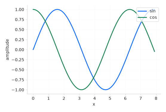
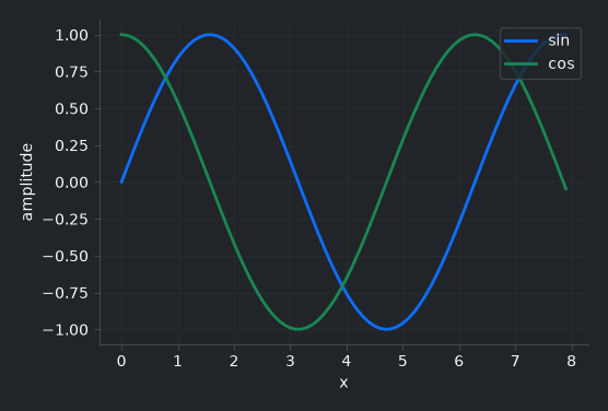
Multiple series are themed automatically: the first line is primary, the second success, and so on, drawn from the theme’s accent colors. The chrome — figure and axes backgrounds, spines, ticks, text — matches the active surface and flips with light/dark, so a bs.toggle_theme() recolors the whole chart with the rest of the app.

Note

matplotlib is an optional dependency. Install it with pip install bootstack[viz]. Build figures with matplotlib’s object API (Figure), never pyplot — an embedded figure must be a standalone object.

Drawing your own figure

If you already have a Figure — or want full control over the styling — hand it over directly. The chart embeds it and recolors only its chrome to the theme; the data series are yours:

from matplotlib.figure import Figure

fig = Figure()
fig.add_subplot(111).plot([1, 2, 3], [4, 5, 6])
bs.Chart(fig, grow=True)

Reach for the managed render path whenever the plot reflects live state — it is what makes the next two guides (signals and data sources) reactive.

Example

def render(ax):
    """Draw two themed series — colors come from the accent cycle."""
    xs = [i / 10 for i in range(80)]
    ax.plot(xs, [math.sin(x) for x in xs], label="sin", linewidth=2)
    ax.plot(xs, [math.cos(x) for x in xs], label="cos", linewidth=2)
    ax.set_xlabel("x")
    ax.set_ylabel("amplitude")
    ax.grid(True, alpha=0.3)
    ax.legend(loc="upper right")


with bs.App(title="Plotting your data", size=(640, 460), padding=16, gap=12) as app:
    bs.Label("Two series, themed to match the app", font="heading-md")
    bs.Chart(render=render, grow=True, horizontal="stretch")
    bs.Button("Toggle theme", on_click=bs.toggle_theme)

app.run()

When to use

This is the foundation. When the plot should update as your state changes, bind a Signal or a data source — see Live and data-driven charts. For statistical plots (bars, boxes, distributions) reach for seaborn — Statistical plots with seaborn. For continuous motion, Real-time and animated charts. The full widget reference is the Chart guide.