Live and data-driven charts

Bind a chart to reactive state so it redraws itself — from a Signal, or from a data source it shares with a table.

How it works

The managed render path becomes reactive the moment you bind a source. Two ways to do it.

From a signal

Pass a Signal and render receives its value; the chart re-renders whenever the signal changes — so any control bound to that signal drives the chart:

count = bs.Signal(20)

def render(ax, n):
    ax.plot(range(n), [i * i for i in range(n)])

bs.Chart(render=render, signal=count, grow=True)
bs.Slider(signal=count, min_value=5, max_value=80)   # drag → chart redraws

From a data source

Pass a data_source and render receives the source’s records (a list of dicts). The chart re-renders whenever the source changes — so a chart and a DataTable on the same source stay in lockstep:

from bootstack.data import MemoryDataSource

ds = MemoryDataSource()
ds.load([{"month": "Jan", "sales": 120}, {"month": "Feb", "sales": 180}])

def render(ax, rows):
    ax.bar([r["month"] for r in rows], [r["sales"] for r in rows])

bs.Chart(render=render, data_source=ds, grow=True)
bs.DataTable(data_source=ds, columns=["month", "sales"])

Insert a record into the source and both views update. The chart reads the source’s current filtered and sorted view, so calling ds.where(...) or ds.order(...) reshapes the plot too:

from bootstack.data import col

ds.where(col("sales") >= 150)   # both the chart and the table follow

Note

matplotlib’s draw() is not free. For a high-frequency source or signal, pass debounce=<ms> to coalesce a burst of changes into one redraw; the chart also skips redraws while it is off-screen.

Example

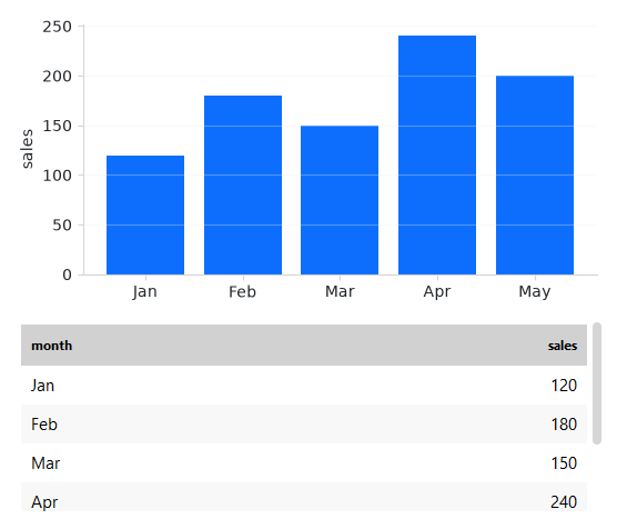
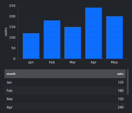
A chart and a table on one source, with a filter toggle and an “add” button — every change flows to both views:

def render(ax, rows):
    """Bar chart of sales by month — `rows` is the source's (filtered) records."""
    ax.bar([r["month"] for r in rows], [r["sales"] for r in rows])
    ax.set_ylabel("sales")
    ax.grid(True, axis="y", alpha=0.3)


with bs.App(title="Live charts", min_size=(680, 620), padding=16, gap=12) as app:
    sales = MemoryDataSource()
    sales.load([
        {"month": "Jan", "sales": 120},
        {"month": "Feb", "sales": 180},
        {"month": "Mar", "sales": 150},
        {"month": "Apr", "sales": 240},
        {"month": "May", "sales": 200},
    ])

    bs.Label("One source, two views — they stay in sync", font="heading-md")
    bs.Chart(render=render, data_source=sales, grow=True, horizontal="stretch")
    bs.DataTable(data_source=sales, columns=["month", "sales"],
                 searchable=False, grow=True, horizontal="stretch")

    high_only = bs.Signal(False)

    def apply_filter(checked):
        # Filtering the SOURCE updates both the chart and the table.
        sales.where(col("sales") >= 180 if checked else None)

    high_only.subscribe(apply_filter)

    state = {"n": 6}

    def add_month():
        n = state["n"]
        state["n"] = n + 1
        sales.insert({"month": f"M{n}", "sales": 100 + (n * 43) % 180})

    with bs.Row(gap=8, horizontal="stretch"):
        bs.Switch("High months only (>= 180)", signal=high_only)
        bs.Spacer()
        bs.Button("Add month", accent="primary", on_click=add_month)

app.run()

When to use

Use signal= when the chart reflects a single reactive value (a control, a computed result); use data_source= when it visualizes records you also show elsewhere. For the data-source model in depth, see Displaying Data and Data Sources. For continuous, high-rate motion, Real-time and animated charts is the better tool than a fast signal.